Here are the Code examples of this chapter. You can compile them online right on this web page by pressing the Typeset / Compile button. You can also edit them for testing, and compile again.
For a better view with the online compiler, I sometimes use \documentclass[border=10pt]{standalone} instead of \documentclass{article}. Instead of having a big letter/A4 page, the standalone class crops the paper to see just the visible text without an empty rest of a page.
Any question about a code example? Post it on LaTeX.org, I will answer. As forum admin I read every single question there. (profile link).
Example document
\documentclass[preview,border=10pt]{standalone}
\begin{document}
\section*{Quadratic equations}
The quadratic equation
\begin{equation}
  \label{quad}
  ax^2 + bx + c = 0,
\end{equation}
where \( a, b \) and \( c \) are constants and \( a \neq 0 \),
has two solutions for the variable \( x \):
\begin{equation}
  \label{root}
  x_{1,2} = \frac{-b \pm \sqrt{b^2-4ac}}{2a}.
\end{equation}
If the \emph{discriminant} \( \Delta \) with
\[
  \Delta = b^2 - 4ac
\]
is zero, then the equation (\ref{quad}) has a double solution:
(\ref{root}) becomes
\[
  x = - \frac{b}{2a}.
\]
\end{document}
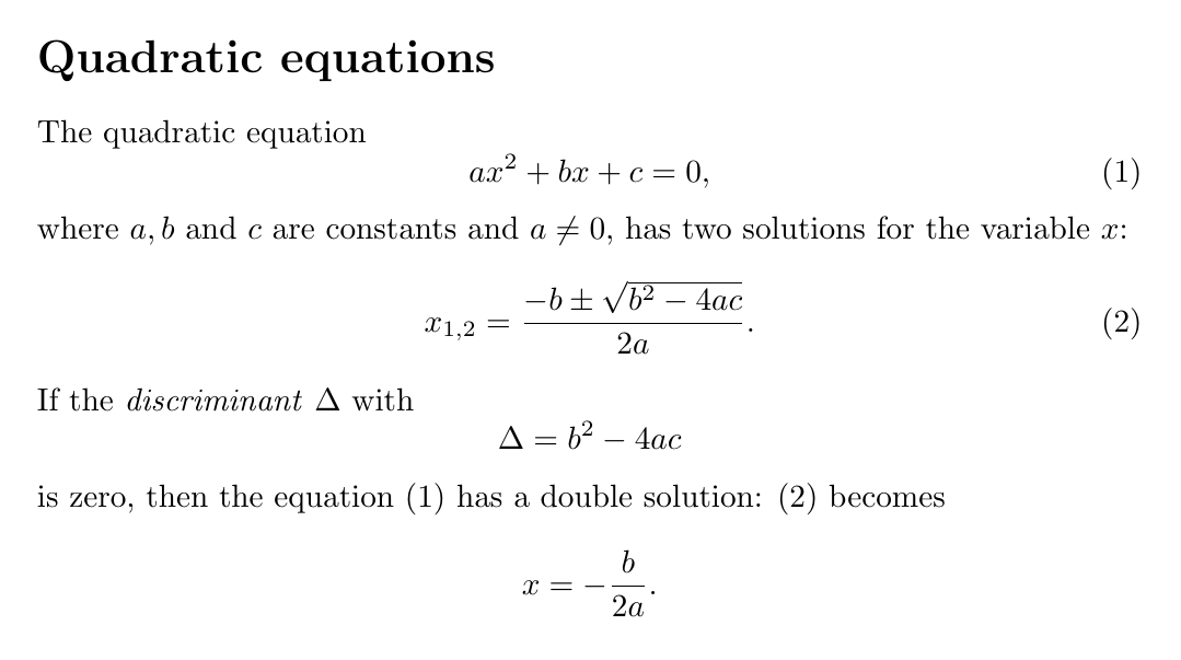
Figure 9.1
Subscripts and superscripts
\documentclass[preview,border=10pt]{standalone}
\begin{document}
\[
  x_1^2 + x_2^2 = 1, \quad 2^{2^x} = 64
\]
\end{document}
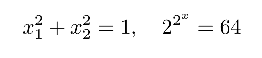
Figure 9.2
Operators
\documentclass[preview,border=10pt]{standalone}
\begin{document}
\[
  \lim_{n=1, 2, \ldots} a_n \qquad \max_{x<X} x
\]
\end{document}
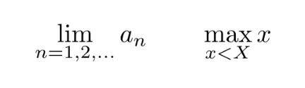
Figure 9.3
Operators within text
\documentclass[preview,border=10pt]{standalone}
\begin{document}
Within text, we have \( \lim_{n=1, 2, \ldots} a_n \)
and \( \max_{x<X} x \).
\end{document}

Figure 9.4
Roots
\documentclass[preview,border=10pt]{standalone}
\begin{document}
\[
  \sqrt[64]{x} = \sqrt{\sqrt{\sqrt{\sqrt{\sqrt{\sqrt{x}}}}}}
\]
\end{document}
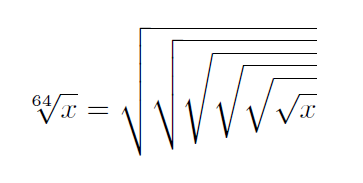
Figure 9.5
Fractions
\documentclass[preview,border=10pt]{standalone}
\begin{document}
\[
  \frac{n(n+1)}{2} \quad \frac{\frac{\sqrt{x}+1}{2}-x}{y^2}
\]
\end{document}
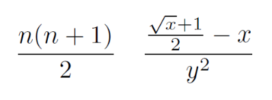
Figure 9.6
Greek letters
\documentclass[border=10pt]{standalone}
\newcommand*\s[1]{$#1$&\texttt{\string#1}}
\setlength{\tabcolsep}{2ex}
\begin{document}
\begin{tabular}{l@{~}ll@{~}ll@{~}ll@{~}ll@{~}l}
\s\alpha      & \s\zeta   &   \s\lambda  & \s\pi     & \s\phi \\
\s\beta       & \s\eta    &   \s\mu      & \s\rho    &\s\chi \\
\s\gamma      & \s\theta  &   \s\nu      & \s\sigma  &\s\psi\\
\s\delta      & \s\iota   &   \s\xi      & \s\tau    &\s\omega \\
\s\epsilon    & \s\kappa  &   \s o       & \s\upsilon&
\end{tabular}
\end{document}
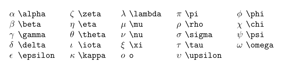
Figure 9.7
Variants of Greek letters
\documentclass[border=10pt]{standalone}
\newcommand*\s[1]{$#1$&\texttt{\string#1}}
\setlength{\tabcolsep}{2ex}
\begin{document}
\begin{tabular}{l@{~}ll@{~}ll@{~}l}
\s\varepsilon & \s\varpi   & \s\varsigma  \\
\s\vartheta   & \s\varrho  & \s\varphi
\end{tabular}
\end{document}
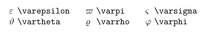
Figure 9.8
Uppercase Greek letters
\documentclass[border=10pt]{standalone}
\newcommand*\s[1]{$#1$&\texttt{\string#1}}
\setlength{\tabcolsep}{2ex}
\begin{document}
\begin{tabular}{l@{~}ll@{~}ll@{~}ll@{~}l}
\s\Gamma &\s\Lambda &\s\Sigma   &\s\Psi   \\
\s\Delta &\s\Xi     &\s\Upsilon &\s\Omega \\
\s\Theta &\s\Pi     &\s\Phi
\end{tabular}
\end{document}
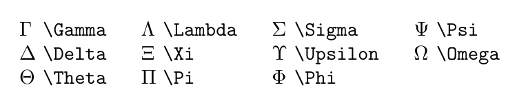
Figure 9.9
Upright Greek letters
\documentclass[border=10pt]{standalone}
\usepackage{upgreek}
\newcommand*\s[1]{$#1$&\texttt{\string#1}}
\setlength{\tabcolsep}{2ex}
\begin{document}
\thispagestyle{empty}
\begin{tabular}{l@{~}ll@{~}ll@{~}ll@{~}ll@{~}l}
\s\upalpha      & \s\upzeta   &   \s\uplambda  & \s\uppi     & \s\upphi \\
\s\upbeta       & \s\upeta    &   \s\upmu      & \s\uprho    &\s\upchi \\
\s\upgamma      & \s\uptheta  &   \s\upnu      & \s\upsigma  &\s\uppsi\\
\s\updelta      & \s\upiota   &   \s\upxi      & \s\uptau    &\s\upomega \\
\s\upepsilon    & \s\upkappa  &   $\mathrm{o}$&\texttt{\string\mathrm\{o\}} & \s\upupsilon&
\end{tabular}
\end{document}
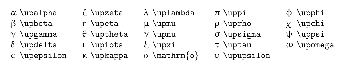
Figure 9.11
Variants of upright Greek letters
\documentclass[border=10pt]{standalone}
\usepackage{upgreek}
\newcommand*\s[1]{$#1$&\texttt{\string#1}}
\setlength{\tabcolsep}{2ex}
\begin{document}
\begin{tabular}{l@{~}ll@{~}ll@{~}l}
\s\upvarepsilon & \s\upvarpi      & \s\upvarsigma  \\
\s\upvartheta   &  \s\upvarrho  & \s\upvarphi
\end{tabular}
\end{document}
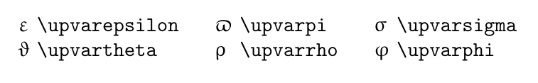
Figure 9.11
Script letters
\documentclass[preview,border=10pt]{standalone}
\begin{document}
\[
  \mathcal{A}, \mathcal{B}, \mathcal{C}, \ldots, \mathcal{Z}
\]
\end{document}
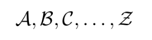
Figure 9.12
Ellipsis
\documentclass[border=10pt]{standalone}
\newcommand*\s[1]{\(#1\)&\texttt{\string#1}}
\setlength{\tabcolsep}{1.8ex}
\begin{document}
\centering
\begin{tabular}{*3{c@{~}l}}
\s\ldots & \s\ddots \\
\s\cdots & \s\vdots \\
\end{tabular}
\end{document}
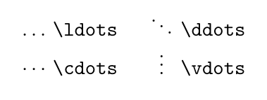
Figure 9.13
Math font styles
\documentclass[border=10pt]{standalone}
\usepackage{booktabs}
\usepackage{amsfonts}
\usepackage{bbm}
\usepackage{dsfont}
\usepackage{eufrak}
\renewcommand*\c{\textbackslash\ttfamily}
\begin{document}
\sffamily
\begin{tabular}{lll}
\toprule
\textbf{Command} & \textbf{Used package} & \textbf{Example} \\
\midrule
\c mathrm\{\ldots\}     &          & \(\mathrm{roman\ 123}\) \\
\c mathit\{\ldots\}     &          & \(\mathit{italic\ 123}\) \\
\c mathsf\{\ldots\}     &          & \(\mathsf{sans-serif\ 123}\) \\
\c mathbb\{\ldots\}     & amsfonts & \(\mathbb{ABC}\)  \\
\c mathbbm\{\ldots\}    & bbm      & \(\mathbbm{C R Q Z 1}\)  \\
\c mathds\{\ldots\}     & dsfont   &\(\mathds{C R Q Z 1}\)  \\
\c mathfrak\{\ldots\}   & eufrak   & \(\mathfrak{A B C \ 1 2 3}\)  \\
\c mathnormal\{\ldots\} &          & \(\mathnormal{normal}\)  \\
\bottomrule
\end{tabular}
\end{document}
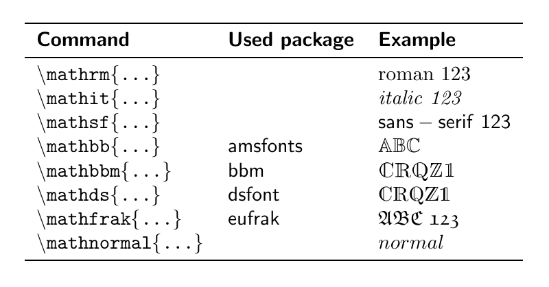
Figure 9.14
Math versus text italic
\documentclass[border=10pt]{standalone}
\begin{document}
\(Definition\) and \textit{Definition}
\end{document}
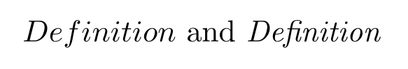
Figure 9.15
Typesetting multi-line formulas
\documentclass[preview,border=10pt]{standalone}
\usepackage{amsmath}
\begin{document}
\begin{multline}
  \sum = a + b + c + d + e \\
           + f + g + h + i + j \\
           + k + l + m + n
\end{multline}
\begin{gather}
  x + y + z = 0 \\
      y - z = 1
\end{gather}
\begin{align}
  x + y + z &= 0 \\
      y - z &= 1
\end{align}
\end{document}
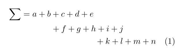
Figure 9.16
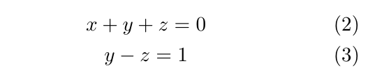
Figure 9.17
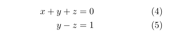
Figure 9.18
Customized tagging
\documentclass[preview,border=10pt]{standalone}
\usepackage{amsmath}
\begin{document}
\begin{align}
  x + y + z &= 0 \tag{$\star$} \\
  y - z &= 1 \tag{$\star\star$}
\end{align}
\end{document}
Binary operation symbols
\documentclass[border=10pt]{standalone}
\newcommand*\s[1]{\(#1\)&\texttt{\string#1}}
\setlength{\tabcolsep}{1ex}
\usepackage{booktabs}
\usepackage{latexsym}
\begin{document}
\sffamily
\centering
\begin{tabular}{*4{c@{~}l}}
\toprule
\multicolumn{8}{c}{\bfseries Standard \LaTeX} \\
\s\amalg           &  \s\circ      & \s\ominus   &   \s\star      \\
\s\ast             &  \s\cup       & \s\oplus    &   \s\times  \\
\s\bigcirc         &  \s\dagger    & \s\oslash   &   \s\triangleleft\\
\s\bigtriangledown &  \s\ddagger   & \s\otimes   &   \s\triangleright \\
\s\bigtriangleup   &  \s\diamond   & \s\pm       &   \s\uplus   \\
\s\bullet          &  \s\div       & \s\setminus &   \s\vee     \\
\s\cap             &  \s\mp        & \s\sqcap    &   \s\wedge   \\
\s\cdot            &  \s\odot      & \s\sqcup    &   \s\wr      \\
\midrule
\multicolumn{8}{c}{\bfseries latexsym }\\
\s\unlhd & \s\unrhd  & \s\rhd & \s\lhd \\
\bottomrule
\end{tabular}
\end{document}
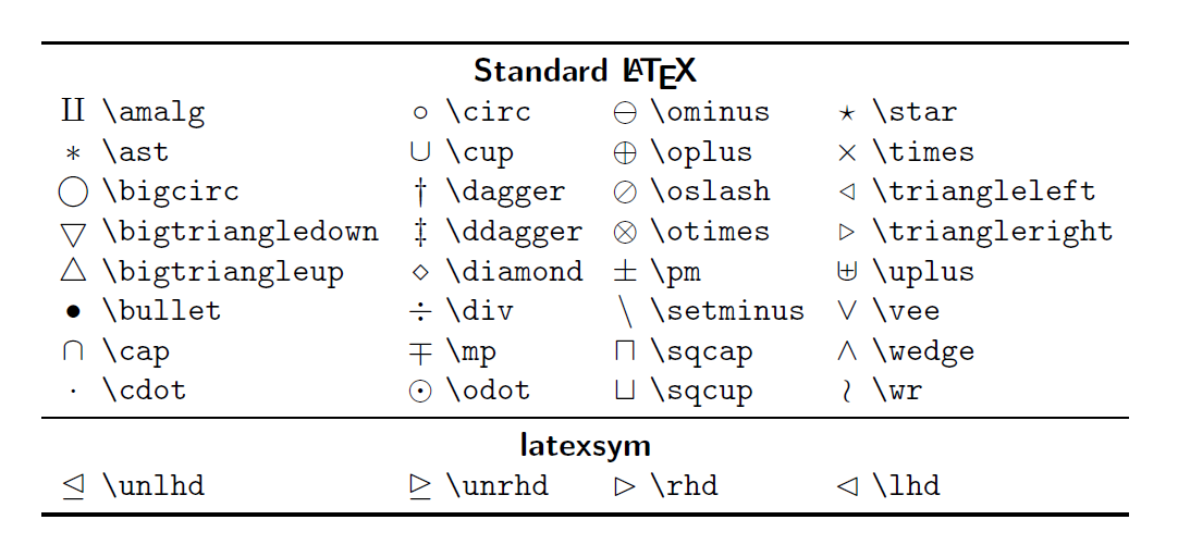
Figure 9.19
Binary relation symbols
\documentclass[border=10pt]{standalone}
\newcommand*\s[1]{\(#1\)&\texttt{\string#1}}
\setlength{\tabcolsep}{1.8ex}
\usepackage{booktabs}
\usepackage{latexsym}
\begin{document}
\begin{tabular}{*4{c@{~}l}}
\toprule
\multicolumn{8}{c}{\bfseries Standard \LaTeX} \\
\s\approx   & \s\equiv    &  \s\prec   & \s\succ \\
\s\asymp    & \s\frown    &  \s\preceq & \s\succeq  \\
\s\bowtie   & \s\mid      &  \s\propto & \s\vdash \\
\s\cong     & \s\models   &  \s\sim    &   \\
\s\dashv    & \s\parallel &  \s\simeq      \\
\s\doteq    & \s\perp     &  \s\smile      \\
\midrule
\multicolumn{8}{c}{\bfseries latexsym }\\
\multicolumn{8}{c}{\(\Join\) ~ \texttt{\string\Join}} \\
\bottomrule
\end{tabular}
\end{document}
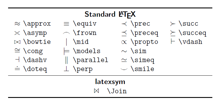
Figure 9.20
Inequality relation symbols
\documentclass[border=10pt]{standalone}
\newcommand*\s[1]{\(#1\)&\texttt{\string#1}}
\setlength{\tabcolsep}{1.8ex}
\usepackage{booktabs}
\begin{document}
\sffamily
\centering
\begin{tabular}{*5{c@{~}l}}
\toprule
\s\geq & \s\gg & \s\leq & \s\ll & \s\neq \\
\bottomrule
\end{tabular}
\end{document}
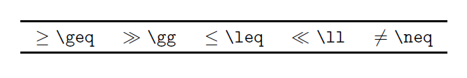
Figure 9.21
Subset and superset symbols
\documentclass[border=10pt]{standalone}
\newcommand*\s[1]{\(#1\)&\texttt{\string#1}}
\setlength{\tabcolsep}{1.8ex}
\usepackage{booktabs}
\usepackage{latexsym}
\begin{document}
\sffamily
\centering
\begin{tabular}{*3{c@{~}l}}
\toprule
\multicolumn{6}{c}{\bfseries Standard \LaTeX} \\
\s\sqsubseteq & \s\subset & \s\supset   \\
\s\sqsupseteq   &  \s\subseteq  & \s\supseteq \\
\midrule
\multicolumn{6}{c}{\bfseries latexsym }\\
\multicolumn{3}{c}{\(\sqsubset\) ~ \texttt{\string\sqsubset}}
& \multicolumn{3}{c}{\(\sqsupset\) ~ \texttt{\string\sqsupset}}\\
\bottomrule
\end{tabular}
\end{document}
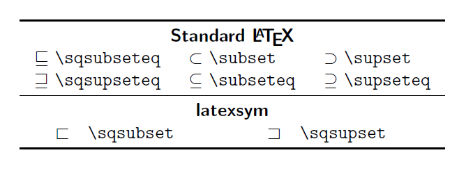
Figure 9.22
Arrows
\documentclass[border=10pt]{standalone}
\newcommand*\s[1]{\(#1\)&\texttt{\string#1}}
\setlength{\tabcolsep}{1.8ex}
\usepackage{booktabs}
\usepackage{latexsym}
\begin{document}
\sffamily
\centering
\begin{tabular}{*3{c@{~}l}}
\toprule
\multicolumn{6}{c}{\bfseries Standard \LaTeX} \\
\s\downarrow       &  \s\Longleftarrow      & \s\Rightarrow   \\
\s\Downarrow       &  \s\longleftrightarrow & \s\searrow   \\
\s\hookleftarrow   &  \s\Longleftrightarrow & \s\swarrow  \\
\s\hookrightarrow  &  \s\longmapsto         & \s\uparrow      \\
\s\leftarrow       &  \s\longrightarrow     & \s\Uparrow  \\
\s\Leftarrow       &  \s\Longrightarrow     & \s\updownarrow   \\
\s\leftrightarrow  &  \s\mapsto             & \s\Updownarrow  \\
\s\Leftrightarrow  &  \s\nwarrow \\
\s\longleftarrow   &  \s\rightarrow \\
\midrule
\multicolumn{6}{c}{\bfseries latexsym }\\
\multicolumn{6}{c}{\(\leadsto\) ~ \texttt{\string\leadsto}}\\
\bottomrule
\end{tabular}
\end{document}

Figure 9.23
Harpoons
\documentclass[border=10pt]{standalone}
\newcommand*\s[1]{\(#1\)&\texttt{\string#1}}
\setlength{\tabcolsep}{1.8ex}
\usepackage{booktabs}
\begin{document}
\sffamily
\centering
\begin{tabular}{*3{c@{~}l}}
%\toprule
\s\leftharpoondown & \s\rightharpoondown & \s\rightleftharpoons \\
\s\leftharpoonup & \s\rightharpoonup \\
%\bottomrule
\end{tabular}
\end{document}
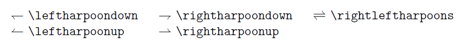
Figure 9.24
Symbols dereived from letters
\documentclass[border=10pt]{standalone}
\newcommand*\s[1]{\(#1\)&\texttt{\string#1}}
\setlength{\tabcolsep}{1.8ex}
\usepackage{booktabs}
\usepackage{latexsym}
\begin{document}
\sffamily
\centering
\begin{tabular}{*5{c@{~}l}}
\toprule
\multicolumn{10}{c}{\bfseries Standard \LaTeX} \\
\s\bot & \s\forall & \s\imath & \s\ni  & \s\top \\
\s\ell & \s\hbar & \s\in  & \s\partial & \s\wp \\
\s\exists & \s\Im  & \s\jmath & \s\Re \\
\midrule
\multicolumn{10}{c}{\bfseries latexsym }\\
\multicolumn{10}{c}{\(\mho\) ~ \texttt{\string\mho}}\\
\bottomrule
\end{tabular}
\end{document}
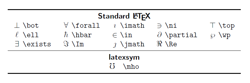
Figure 9.25
Misc symbols
\documentclass[border=10pt]{standalone}
\newcommand*\s[1]{\(#1\)&\texttt{\string#1}}
\setlength{\tabcolsep}{1.8ex}
\usepackage{booktabs}
\usepackage{latexsym}
\begin{document}
\sffamily
\centering
\begin{tabular}{*4{c@{~}l}}
\toprule
\multicolumn{8}{c}{\bfseries Standard \LaTeX }\\
\s\aleph      &  \s\emptyset  &  \s\nabla  &  \s\sharp  \\
\s\angle      &    \s\flat  &\s\natural  & \s\spadesuit  \\
\s\clubsuit   &  \s\heartsuit & \s\neg   &  \s\surd \\
\s\diamondsuit & \s\infty  &\s\prime  &  \s\triangle \\
\midrule
\multicolumn{8}{c}{\bfseries latexsym}\\
\multicolumn{4}{c}{\(\Box\) ~ \texttt{\string\Box}}
& \multicolumn{4}{c}{\(\Diamond\) ~ \texttt{\string\Diamond}}\\
\bottomrule
\end{tabular}
\end{document}
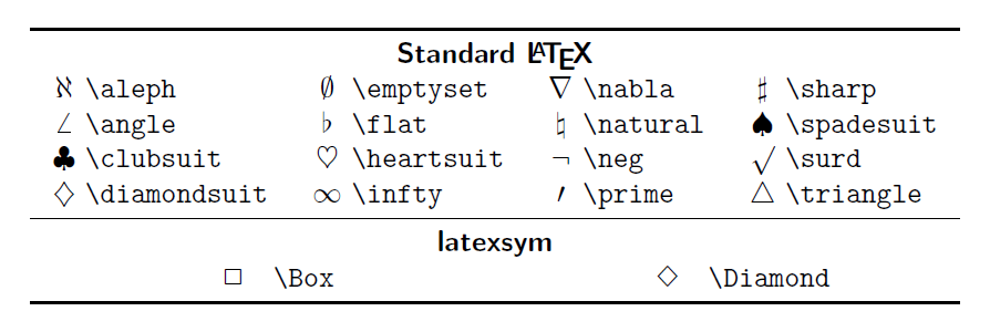
Figure 9.26
Variable sized operators
\documentclass[border=10pt]{standalone}
\newcommand*\s[1]{$\displaystyle#1$&\texttt{\string#1}}
\renewcommand*\arraystretch{1.8}
\setlength{\arraycolsep}{3ex}
\begin{document}
\begin{tabular}{*4{c@{~}l}}
\s\bigcap    & \s\bigotimes & \s\bigwedge  & \s\prod      \\
\s\bigcup    & \s\bigsqcup  & \s\coprod    & \s\sum       \\
\s\bigodot   & \s\biguplus  & \s\int       \\
\s\bigoplus  & \s\bigvee    & \s\oint      \\
\end{tabular}
\end{document}
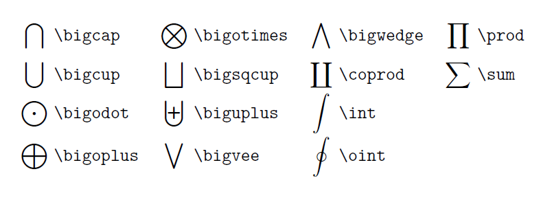
Figure 9.29
Inline text equation
\documentclass[border=10pt]{standalone}
\usepackage{amsmath}
\begin{document}
\(
  \int_a^b \! f(x) \, dx = \lim_{\Delta x \rightarrow 0}
  \sum_{i=1}^{n} f(x_i) \,\Delta x_i
\)
\end{document}
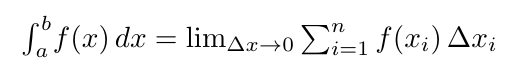
Figure 9.30
Displayed style equation
\documentclass[preview,border=10pt]{standalone}
\usepackage{amsmath}
\begin{document}
\[
  \int_a^b \! f(x) \, dx = \lim_{\Delta x \rightarrow 0}
  \sum_{i=1}^{n} f(x_i) \,\Delta x_i
\]
\end{document}
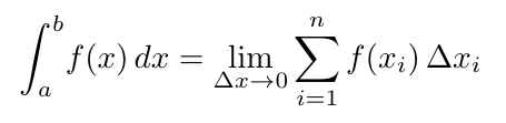
Figure 9.31
Variable sized delimiters
\documentclass[border=10pt]{standalone}
\newcommand*\s[1]{$\displaystyle\Big#1$&\texttt{\string#1}}
\renewcommand*\arraystretch{1.8}
\setlength{\tabcolsep}{2ex}
\usepackage{booktabs}
\begin{document}
\begin{tabular}{*3{c@{\quad}l}}
\toprule
\multicolumn{6}{c}{\bfseries Pairs of braces, brackets  and parentheses} \\
\(\Big(\ \Big)\) & \verb|( )| & \(\Big\{\ \Big\}\) & \verb|\{ \}| & \(\Big\lceil\ \Big\rceil\) & \verb|\lceil \rceil|\\
\({\Big[\ \Big]}\) & \verb|[ ]|  & \(\Big\langle\ \Big\rangle\) & \verb|\langle \rangle|& \(\Big\lfloor\ \Big\rfloor\) & \verb|\lfloor \rfloor| \\
\midrule
\multicolumn{6}{c}{\bfseries Delimiting symbols and arrows}\\
\s/ & \s\downarrow & \s\updownarrow \\
\s\backslash & \s\Downarrow & \s\Updownarrow\\
\s| & \s\uparrow \\
\s\| &  \s\Uparrow \\
%\s\unlhd & \s\unrhd  & \s\rhd & \s\lhd \\
\bottomrule
\end{tabular}
\end{document}
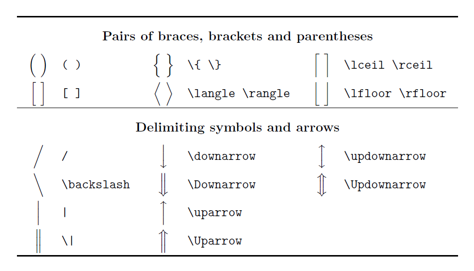
Figure 9.32
Arrays
\documentclass[preview,border=10pt]{standalone}
\usepackage{amsmath}
\begin{document}
\[
  A = \left(
    \begin{array}{cc}
      a_{11} & a_{12} \\
      a_{21} & a_{22}
    \end{array}
  \right)
\]
\end{document}
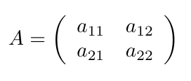
Figure 9.33
Typesetting matrices
\documentclass[preview,border=10pt]{standalone}
\usepackage{amsmath}
\begin{document}
\[
  A = \begin{pmatrix}
    a_{11} & a_{12} \\
    a_{21} & a_{22}
  \end{pmatrix}
\]
\end{document}
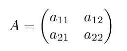
Figure 9.34
Writing binomial coefficients
\documentclass[preview,border=10pt]{standalone}
\usepackage{amsmath}
\begin{document}
\[
\binom{n}{k} = \frac{n!}{k!(n-k)!}
\]
\end{document}
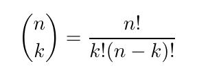
Figure 9.35
Underlining and overlining
\documentclass[preview,border=10pt]{standalone}
\usepackage{amsmath}
\begin{document}
\[
\overline{\Omega}
\]
\end{document}

Figure 9.36
An underbrace below an expression
\documentclass[preview,border=10pt]{standalone}
\usepackage{amsmath}
\begin{document}
\[
N = \underbrace{1 + 1 + \cdots + 1}_n
\]
\end{document}
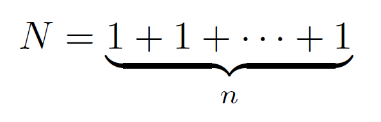
Figure 9.37
Accents
\documentclass[border=10pt]{standalone}
\setlength{\tabcolsep}{1.8ex}
\usepackage{array}
\usepackage{booktabs}
\begin{document}
\sffamily
\centering
\begin{tabular}{*4{>{$}c<{$}@{~}l}}
\toprule
\acute{a} & \verb|\acute{a}| &\check{a} & \verb|\check{a}| &\grave{a} & \verb|\grave{a}| &\tilde{a} & \verb|\tilde{a}| \\
\bar{a} & \verb|\bar{a}|  & \ddot{a} & \verb|\ddot{a}| & \hat{a} & \verb|\hat{a}| & \vec{a} & \verb|\vec{a}|   \\
\breve{a} & \verb|\breve{a}| & \dot{a} & \verb|\dot{a}| & \mathring{a} & \verb|\mathring{a}| \\
\midrule
\multicolumn{8}{c}{\textbf{Extensible}} \\
\multicolumn{4}{c}{$\widehat{abc}$\,\ \texttt{\string\widehat\{abc\}}} & \multicolumn{4}{c}{$\widetilde{abc}$\,\ \texttt{\string\widetilde\{abc\}}}\\
\bottomrule
\end{tabular}
\end{document}
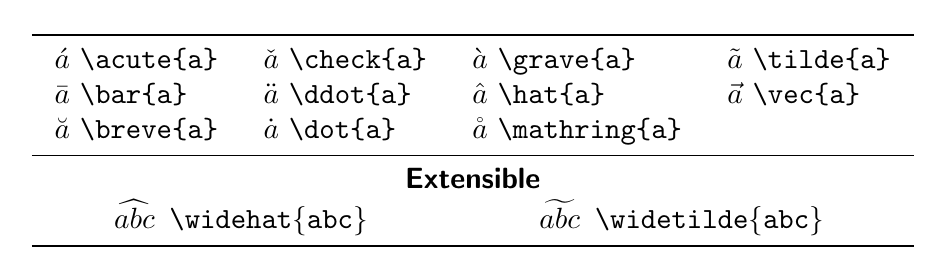
Figure 9.38
Putting a symbol above or below another one
\documentclass[preview,border=10pt]{standalone}
\usepackage{amsmath}
\begin{document}
\[
  \underset{\circ}{\cap} \neq \overset{\circ}{\cup}
\]
\end{document}
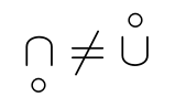
Figure 9.39
Text above a relation symbol
\documentclass[preview,border=10pt]{standalone}
\usepackage{amsmath}
\begin{document}
\[
 X \stackrel{\text{def}}{=} 0
\]
\end{document}
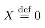
Figure 9.40
Writing theorems and definitions
\documentclass[preview,border=10pt]{standalone}
\usepackage{amsmath}
\newtheorem{thm}{Theorem}
\newtheorem{dfn}[thm]{Definition}
\begin{document}
\begin{dfn}
  A quadratic equation is an equation of the form
  \begin{equation}
    \label{quad}
    ax^2 + bx + c = 0,
  \end{equation}
  where \( a, b \) and \( c \) are constants and \( a \neq 0 \).
\end{dfn}
\begin{thm}
  A quadratic equation (\ref{quad}) has two solutions for the
  Variable \( x \):
  \begin{equation}
    \label{root}
    x_{1,2} = \frac{-b \pm \sqrt{b^2-4ac}}{2a}.
  \end{equation}
\end{thm}
\end{document}
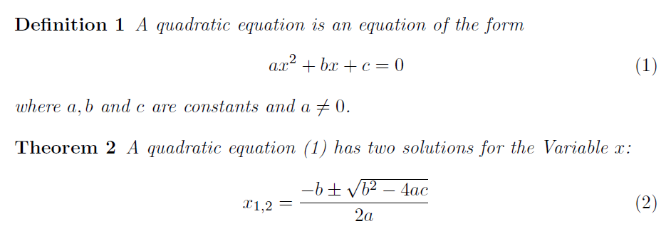
Figure 9.41
This code is available on Github. It is licensed under the MIT License, a short and simple permissive license with conditions only requiring preservation of copyright and license notices.
Go to next chapter.